
 North east of Ukraine, close to the Russian border, is the site of the Duga radar, also known during the 70s and 80s as the Woodpecker – one of the most extraordinary engineering structures ever built.
Today, this giant lattice of steel beams and cables looms silent over the horizon, except perhaps for the eerie creaking of its metallic structure in the wind. Decades ago, this incredible feat of radio engineering could be heard all around the World.
This massive radar antenna is the Duga ‘Woodpecker’.
Basic Radars for Dummies
A radar is a detection system that uses radio waves to determine:
-
- the distance,
- the angle, and
- the radial velocity of any object relative to the radar itself.
It can be used to detect anything from aircraft and seafaring ships, to problematic weather formations.

Basically, a radar transmitter emits continuous or pulsed radio waves that reflect off any object in their path in order to return to the radar receiver, providing the operator with information about the location and speed of the object.
The radar signals that are reflected back towards the radar receiver are the ones that make radar detection work.
Wave Propagation and Radar Frequencies
 In radio technology, the frequency affects the propagation range of the wave.
The higher the frequency, the shorter the wavelength.
As a result,
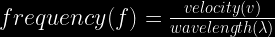
or
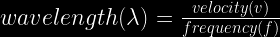
It’s an inverse relationship.
So the higher the frequency, the bigger the buildings and trees appear to the wave. And the more of the radio wave is lost in penetrating them.

The primary wave will travel in a relative straight line from radio transmitter to receiver. Aberrant signals transmitted simultaneously can follow different paths before reaching a receiver, especially if there are obstructions affecting the Fresnel zone.
Hills cause shadows, and the curvature of the Earth also has an effect in making any hills in the middle of the propagation path seem taller.
At VHF or very high frequencies (30 MHz to 300 MHz), the range is not much further than a line-of-sight propagation as seen from the antenna and ignoring small obstructions.
And that is even truer at UHF or ultra high frequencies (300 MHz to 1 GHz).

Depending on the terrain, the range can mean anything from 10 – 20 km and up to 60 – 80 km in open country and from a hilltop.
Radar frequency bands in the microwave range are designated by letters – a convention that began around World War II with military designations for frequencies used in radars.
Frequency Modulation and Doppler Effect
Radar receivers are usually based at the same location as radar transmitters.
Using frequency modulation allows the range of the object to be determined.
If the object is moving either toward or away from the transmitter, there will be a frequency shift of the radio waves due to the Doppler effect or Doppler shift – the change in frequency of a wave in relation to an observer who is moving relative to the wave source.
 A change in the frequency is caused by the motion of the object that changes the number of wavelengths between the reflector and the radar receiver.
Let the object move at a speed v.
Let the frequency transmitted by the radar be fc.
So, the received frequency is either

or
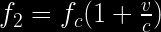
![]()
So the Doppler effect can either degrade or enhance a radar performance, depending upon how it affects the detection process.
The Duga Radar or “Woodpecker”
A decaying relic of the Cold War, the Duga (meaning ‘arc’ or ‘curve’ in Russian) radar system was formerly at the cutting-edge of technology.

The size of the Duga-1 antennas near Chernobyl is a massive 700 metres (2,300 ft) long and 150 metres (490 ft) high. In its heyday, NATO military intelligence gave it the reporting name STEEL YARD.
The project was shrouded in secrecy. On Soviet maps, the Duga radar was marked as a children’s camp.
It is thought that its first broadcast was in 1976. Duga-1 was aimed northward and covered the continental United States.

But there were other woodpeckers.
The experimental prototype for Duga was built in the south of what is now Ukraine near Mykolaiv.
And in the Russian far east, there was Duga-2.
Duga-3 does not exist.
Giant antenna arrays were not a new thing when the Duga radar was constructed in the 1970s.
In the mid-1950s, the Americans built the Distant Early Warning (DEW) Line. Essentially, DEW was a string of litterally dozens of radar installations in the far north of Canada.
However, those were essentially line-of-sight radars.
And no matter how high up a mountain you can set up your antenna, you can never get much more than a 100 km + range under the best conditions.
Line-of-Sight Radio Propagation
 The line-of-sight propagation characteristics of an electromagnetic wave means that waves can travel in a direct path from the source to the receiver.
Unfortunately, the Earth is round.
The Earth bulge limits the distance any wave can travel to the horizon.
Besides, any groundwave radio propagation gives a rapidly decaying signal at increasing distances over ground.
For this reason, in the VHF and UHF bands, the propagation range is no farther than the line-of-sight.
For this reason, such broadcast stations have a limited range.
Duga Radar and the Ionosphere
The Duga radar system was different.
It was created to make use of the ionosphere.
Ionosphere

The ionosphere is the region of the upper atmosphere of Earth, from about 48 km (30 mi) to 965 km (600 mi) above sea level (ASL).
It is an atmospheric region that includes the thermosphere and parts of the mesosphere and exosphere.
This layer comprises vast amounts of charged particles or ions, also referred to as plasma. It plays an important role in atmospheric electricity and forms the inner edge of the magnetosphere.

It is ionized by solar radiation, and it is the reason aurorae occur.
The ionosphere has a practical importance because, amongst other things, it influences radio propagation to distant places on Earth.
However, irregularities in the layer make it difficult or impossible to triangulate objects accurately without the back up of modern computing power.
To overcome the radio horizon limit, the idea of Over-The-Horizon radars (OTH) came about in the late 1940s.
OTH radars give you the ability to scan an area thousands of kilometres in range.
It’s quite possible that the Duga radar system may have been used to eavesdrop on the United States to detect long-range missile launches.
Over-The-Horizon Radar Systems
 If you want to detect things that are beyond the horizon, you need to make the wave bend.
In other words, “Eureka!”
The wave has to go around the curvature of the Earth.
One of the ways to bend the wave, is with the ionosphere and some low to medium frequencies.
Plasma Frequency
Here we can briefly talk about plasma frequency because it controls what frequency of electromagnetic radiation will be transmitted through each layer of the ionosphere.
 When waves of radiation pass through free electrons, the electrons respond by moving.
In turn, the very motion of the electrons generate their own electromagnetic field.
But if the transmitted frequency is higher than the plasma frequency, the electrons cannot respond fast enough and cannot generate their own electromagnetic field.
In this case, the transmitted radio waves can pass through the electrons unimpeded.
However, if the radar is transmitting at a lower frequency than the the plasma frequency, then the energy from the transmitted radiation is absorbed by the electrons, causing them to vibrate at that frequency.
This process generates new electromagnetic waves in the opposite direction to the original transmission.
Under this scenario, the effect of the free electrons is to reflect the radio transmission back down toward the surface of the Earth.
Radar Transmission Frequencies
The critical frequency is always within the high frequency (HF) range.
At high frequency (3 MHz to 300 MHz), the radio waves are above the Penetration Threshold (MUF) – the maximum usable frequency.
At medium frequency (300 kHz to 3 MHz), the waves are suitable for Skip.

Between frequency “hops”, are the “skip zones“. In these regions, the signal is weak or nonexistent.
The higher skip zones may have stronger signals than the first one because rays at different transmission angles tend to spread out and fill in these gaps.
At low frequency (30 kHz to 300 kHz), the waves are below the Absorption Threshold (LUF) – the lowest usable frequency.
They cannot go through the ionosphere, so they literally just bounce off it.
Phased Array Radars
Normal radars transmit one beam of energy at a time. They listen for the returned energy, then the radar mechanically tilts up a little higher, and samples another small section of the atmosphere.
When it has sampled the entire volume of atmosphere, from bottom to top at a particular location, the radar goes back down, moves over a little, and starts the process all over again.
This procedure continues until the radar has scanned the entire atmosphere, which can take around 6 or 7 minutes.
Not all radar antennas need rotating to scan the sky.

A phased array radar has a unique antenna that collects the same information as a conventional radar in about one-sixth the time.
The radar’s electronic beams can be directed independently at particular objects or elements of a storm to give forecasters more accurate and complete data.
Phased arrays use multiple beams sent out at one time. The antennas never need to tilt. Scanning the horizon takes only 30 seconds, and it already has dual-polarization capabilities.
Radar Components
A phased array radar system consists of
- an array of antenna elements (A) powered by
- a transmitter (TX).
The feed current for each element passes through
- a phase shifter (φ) controlled by
- a computer (C).
The individual wavefronts are spherical, but they combine (i.e. they superpose) in front of the antenna to create a plane wave, a beam of radio waves travelling in a specific direction.
Electromagnetic plane waves are strictly transverse waves since their oscillations are perpendicular to the direction of propagation.
Phase Modulation

In phase modulation, the instantaneous amplitude of the baseband signal modifies the phase of the carrier signal keeping its amplitude and frequency constant.
The phase of a carrier signal is modulated to follow the changing signal level (amplitude) of the message signal.
Radar phase shifters delay the radio waves progressively going up the line so each antenna emits its wavefront later than the one below it.
This causes the resulting plane wave to be directed at an angle θ to the antenna’s axis.
By changing the phase shifts, the computer can instantly change the angle θ of the beam.
There are two regions of particular interest in phase modulation:
-
- For small amplitude signals, phase modulation is similar to amplitude modulation (AM) and exhibits its unfortunate doubling of baseband bandwidth and poor efficiency.
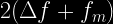
- For a single large sinusoidal signal, phase mpdulation (PM) is similar to frequency modulation (FM) and its bandwith can be approximated by Carson’s Rule:
Radar Scanning Procedures
With different scanning strategies , you can monitor simultaneously multiple objects of interest in the environment:
- Electronic beam steering applications to maximize weather observations
-
- Allow a beam to follow the terrain to minimize ground clutter
- Can notch out various buildings/structures to minimize radio frequency exposure where required
- Allow a quick surveillance scan, and then a return to the targets that are most important to obtain fine-scale data with improved space and time resolution
- Could be designed to concentrate on various phenomena such as precipitation measurements and wind measurements
- Radial-by-radial processing will allow more flexibility in displaying and processing the data with algorithms.
- Beam multiplexing will improve scanning speed by using the radarsphased array antenna’s electronic beam steering capability.
- Pulse compression will combine the high energy of a long pulse with the high resolution of a short pulse to allow the radar to “see” farther.
Active Phased Arrays and Military Defence
Active phased arrays are an even more advanced, second-generation phased-array technology used in military applications.
Unlike PESA (Phased Electronically Scanned Arrays) radars, AESA radars can radiate several beams of radio waves at multiple frequencies in different directions simultaneously.

Researchers believe phased arrays extend warning lead times from 10 minutes to 18-22 minutes.
In an active phased array, each antenna element has an analog transmitter/receiver (T/R) module which creates the phase shifting required to electronically steer the antenna beam.
The massive structure of the Duga radar formed a phased array, necessary to provide high gain at HF, as well as facilitating beam-steering.
At the time of its construction, the World was a very different place.
During the Cold War, people were spooked. Nations were on edge. For the Soviet Union, the anticipated enemy was known to be from the West and they really wanted to have this early warning protection system.
With its ability to detect incoming missiles, the Duga radar system was at the frontline of any future war. But would it have worked?
We understand the ionosphere is not a smooth atmospheric layer. Therefore, there are many ways a radar signal can bounce off it.
The Soviets knew that any potential missile would take only minutes to reach their target. Speedy accurate readings of incoming signals would have been essential.
Without adequate computing power, however, it would have greatly complicated the accurate determination of an object, and left the Duga system subject to human error, which in those days of international paranoia could have quickly spelt disaster for the entire World.
Ham Radio and The Woodpecker
 Although it is now widely known about, the Duga radar was a closely guarded secret during its years of operation.
And yet, as early as 1963, ham radio operators were calling this type of radio signal the “Russian Woodpecker”.
In 1976, a powerful new radio signal appeared, which was simultaneoulsy detected worldwide. It was quickly nicknamed the “Woodpecker” or the “Machine Gun” by the amateur radio community because it sounded like sharp, repetitive tapping noises at a frequency of 10 Hz.
Duga-1 was letting the World know it was on:
Although little is known about its power levels, it was probably a forerunner of the Duga radar systems.
The transmission power on some woodpecker transmitters was estimated to be as high as 10 MW.
On the other hand, Duga must have had the computing power of any early processor in the 1970s, which by today’s standards was minuscule.

However, for all that, its signal was no less of a nuisance largely due to its interference with certain long-range air-to-ground communications systems used by commercial airliners.
The random frequency hops often disrupted legitimate broadcasts, ham radio operations, oceanic commercial aviation communications and utility transmissions, resulting in thousands of complaints from many countries worldwide.
Data analysis showed a pulse repetition interval (PRI) of about 90 ms, a frequency range of 7 to 19 MHz, a bandwidth of 0.02 to 0.8 MHz, and typical transmission time of 7 minutes.
The pulses transmitted by the Duga Woodpecker had a wide bandwidth, typically 40 kHz. Their repetition frequencies were 10 Hz, 16 Hz and 20 Hz, with the most common frequency of 10 Hz.
Hunting for Woodpeckers
To combat this interference, amateur radio operators attempted to jam the signal by transmitting synchronized unmodulated continuous wave signals at the same pulse rate as the offending signal. They were The Russian Woodpecker Hunting Club.
The signal became such a nuisance that communications receivers began including “Woodpecker Blankers” in their circuit designs.
Eventually, the Soviet Union shifted the frequencies they used, without admitting they were even the source.
While the ham radio community was well aware of the system, the OTH theory was not publicly confirmed until after the dissolution of the Soviet Union.
Like all such radar installations, the construction and operation of the Duga-1 project was shrouded in secrecy, but when the nearby Chernobyl power station went offline in 1986, it lost its power source and its entire complex was abandoned seemingly overnight.
Equipment and technology associated with the radar was either ransacked or returned to Russia after the collapse of the Soviet Union.

Now, the giant that could have started World War III is rusting away in the contaminated zone around Chernobyl, just north of Kiev. Too costly to demolish and impossible to re-use.
The Duga’s exact purpose was never fully understood…
And today, the Russian woodpecker is silent. Or is it…? What is this spooky repeating signal on this random frequency…?
No. Just another data station…
You must be logged in to post a comment.